Creating a Budget with Google Sheets: A Step-by-Step Guide
A budget is a crucial tool for managing your finances and reaching your financial goals. Whether you’re saving for a down payment on a house, paying off debt, or simply trying to spend wisely, a budget can help you track your spending and stay on track. In this article, we’ll walk you through the steps for creating a budget with Google Sheets.
Step 1: Set up your sheet
The first step in creating a budget with Google Sheets is to set up your sheet. Start by creating a new sheet, or use an existing one that you’ve already set up.
Next, decide what data you want to track. Some common pieces of information that you might want to include are:
- Date
- Description
- Category (e.g. “Housing,” “Transportation,” “Entertainment”)
- Payment method (e.g. “Cash,” “Credit card,” “Debit card”)
- Amount
Create a column for each piece of data that you want to track, and give each column a descriptive title.
Step 2: Enter your data
Once you’ve set up your sheet, it’s time to enter your data. In each row, add a new transaction and fill in the relevant information for that transaction.

Step 3: Use formulas to calculate your budget
Google Sheets includes a variety of formulas that you can use to calculate your budget. For example, you might want to use a formula to calculate your total income and expenses for a given period of time.
To do this, create a new sheet in your budget workbook, and give it a descriptive name (e.g. “Summary”). In the first row of the summary sheet, create columns for “Category,” “Income,” and “Expenses.”
Next, in the “Category” column, enter the names of the categories that you want to track (e.g. “Housing,” “Transportation,” “Entertainment”).
In the “Income” column, enter a formula to sum the income for each category. For example, if your income data is in a sheet called “Transactions,” and you want to sum the income for the “Income” category, you might use a formula like this:
=SUMIF(Transactions!D:D, “Income”, Transactions!E:E)
This formula will sum all of the values in the “Amount” column (E) where the corresponding value in the “Category” column (D) is “Income.”
Repeat this process for each of the categories that you want to track.
In the “Expenses” column, use a similar formula to sum the expenses for each category. For example:
=SUMIF(Transactions!D:D, “Housing”, Transactions!E:E)
This formula will sum all of the values in the “Amount” column where the corresponding value in the “Category” column is “Housing.”
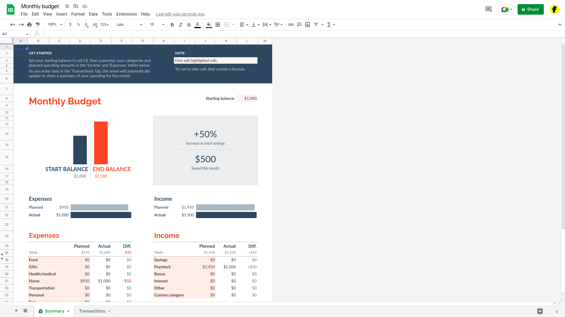
Step 4: Use charts to visualize your budget
Google Sheets includes a variety of chart types that you can use to visualize your budget data. To create a chart, select the data that you want to include in the chart, then click the “Insert” dropdown in the toolbar and select “Chart.”
Choose the chart type and style that you want to use, then click “Insert” to add the chart to your sheet. You can then customize the chart by clicking on it and using the options in the toolbar.
Conclusion:
By following these steps, you can create a budget with Google Sheets that will help you track your income and expenses and stay on track with your financial goals. Whether you’re working on a personal budget or a budget for a business or organization, Google Sheets is a powerful and flexible tool that can help you manage your finances effectively.


