How to Use Conditional Formatting in Google Sheets: A Step-by-Step Guide

Conditional formatting is a powerful tool in Google Sheets that allows you to apply formatting to cells based on certain conditions. This can be a great way to visually highlight important information or draw attention to trends in your data. In this guide, we’ll walk you through the steps for using conditional formatting in Google Sheets.

You can access this sheet here.

Step 1: Select the cells that you want to apply formatting to.

To begin, select the cells that you want to format. This can be a single cell, a range of cells, or an entire column or row. To select a single cell, simply click on it. To select a range of cells, click and drag your mouse over the cells that you want to include. To select an entire column or row, click on the letter or number at the top or left of the column or row.

Step 2: Open the conditional formatting menu.

Next, click the “Format” dropdown in the toolbar at the top of the screen. From the dropdown menu, select “Conditional formatting.” This will open the conditional formatting options on the right side of the screen.

Step 3: Choose the formatting conditions.

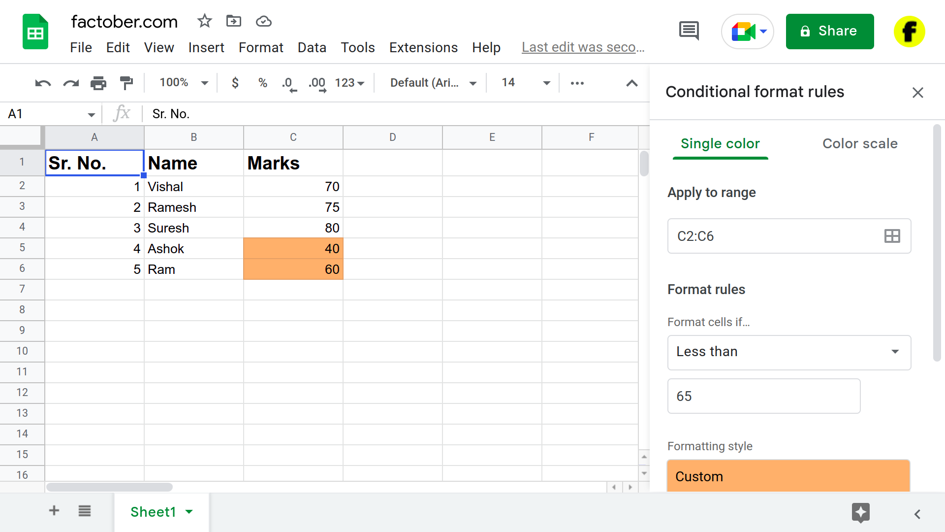
In the “Format cells if” dropdown, choose the condition that you want to trigger the formatting. There are several options to choose from, including “Less than,” “Greater than,” and “Between.” You can also use a custom formula to specify more complex conditions. To do this, select “Custom formula is” in the dropdown and enter your formula in the field provided.

Step 4: Select the formatting style.

Once you’ve chosen your formatting conditions, select the formatting that you want to apply from the dropdown menu under “Formatting style.” You can choose from a variety of options, including font color, background color, and cell borders.

Step 5: Add additional formatting rules (optional).

You can add additional formatting rules by clicking the “Add another rule” button. This allows you to specify multiple conditions and formatting styles for your cells. For example, you might want to use one color for cells with a value less than 50 and another color for cells with a value greater than 50.

Step 6: Apply the formatting.

When you’re finished adding rules, click the “Done” button to apply the formatting to your selected cells.

That’s it! You now know how to use conditional formatting in Google Sheets. Whether you’re working with data, creating a spreadsheet for personal use, or collaborating with others, this handy tool can help you quickly and easily highlight important information and make your data more visually appealing.