5 Advanced Formulas Every Google Sheets User Should Know

Google Sheets includes a wide variety of formulas that can be used to perform a wide range of calculations. While basic formulas like SUM and AVERAGE are useful for many purposes, there are also a number of advanced formulas that can be very powerful tools for data analysis and manipulation.

Formula 1: IFERROR

The IFERROR formula allows you to specify what should happen if an error occurs when evaluating a formula. This can be useful for handling errors that might occur due to missing or invalid data.

For example, consider the following formula:

=AVERAGE(A1:A10)

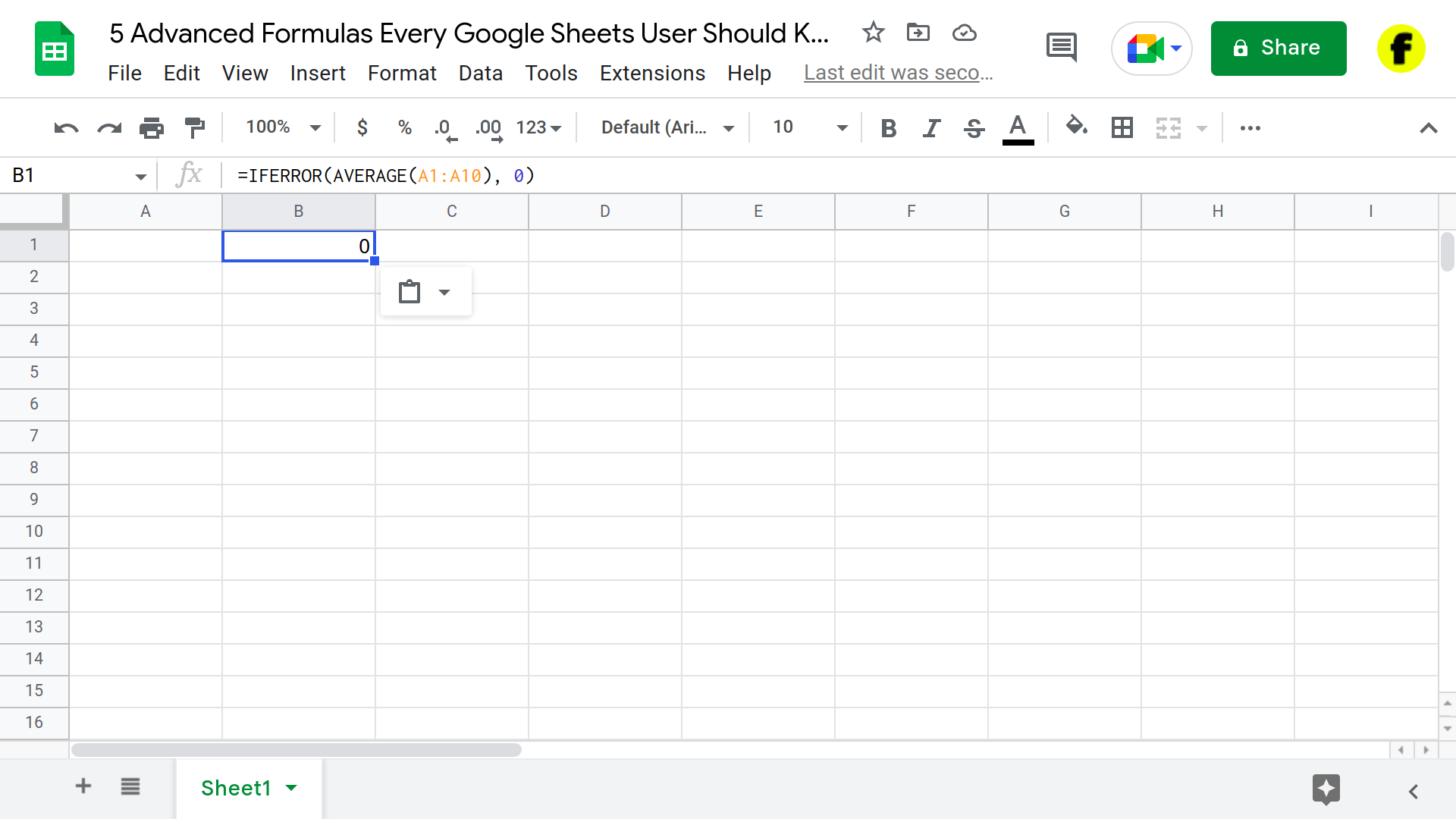
If any of the cells in the range A1:A10 contain an error, this formula will return an error as well. To handle this error and return a different value, you can use the IFERROR formula like this:

=IFERROR(AVERAGE(A1:A10), 0)

This formula will return 0 if an error occurs when calculating the average, rather than returning an error.

Formula 2: INDEX and MATCH

The INDEX and MATCH formulas can be used together to perform advanced lookups in Google Sheets. While the VLOOKUP formula is often used for this purpose, INDEX and MATCH offer more flexibility and can be more efficient in some cases.

Here’s an example of how to use INDEX and MATCH to look up a value in a table:

=INDEX(B1:D10, MATCH(“Apple”, A1:A10, 0), MATCH(“Price”, B1:D1, 0))

This formula will look for the value “Apple” in the range A1:A10 and return the value in the same row, but in the column where the heading “Price” is located.

Formula 3: SUMIFS and COUNTIFS

The SUMIFS and COUNTIFS formulas allow you to sum or count cells based on multiple criteria. This can be useful for performing calculations on specific subsets of your data.

For example, consider the following formula:

=SUMIFS(E1:E10, A1:A10, “Apple”, B1:B10, “Red”)

This formula will sum all of the values in the range E1:E10 where the corresponding cells in the range A1:A10 are “Apple” and the corresponding cells in the range B1:B10 are “Red.”

Formula 4: NETWORKDAYS

The NETWORKDAYS formula allows you to calculate the number of working days between two dates, excluding weekends and holidays. This can be useful for tasks such as estimating project duration or calculating deadlines.

Here’s an example of how to use the NETWORKDAYS formula:

=NETWORKDAYS(A1, B1, C1:C5)

This formula will calculate the number of working days between the dates in cells A1 and B1, excluding the dates in the range C1:C5 (which should contain a list of holidays).

Formula 5: TRANSPOSE

The TRANSPOSE formula allows you to transpose (i.e., flip) a range of cells, converting rows into columns and vice versa. This can be useful for rearranging data or combining data from multiple sources.

Here’s an example of how to use the TRANSPOSE formula:

=TRANSPOSE(A1:E5)

This formula will transpose the range A1:E5, converting the rows into columns and the columns into rows.

Conclusion

By mastering these advanced formulas, you’ll be able to perform a wide range of calculations and manipulations with Google Sheets. Whether you’re working with large data sets, performing complex lookups, or simply trying to make sense of your data, these formulas can help you get more out of your data and work more efficiently with Google Sheets. So, these are the 5 advanced formulas that every Google Sheets user should know.